GEOSPATIAL ASSESSMENTS FOR CWIS PLANNING

• Assessments of Hard to Reach (HTR) Settlements
• Stepwise Process Flow Details
• Output Application
• Assessments of Waterlogging/Flood Prone Settlements
• Stepwise Process Flow Details
• Output Application
• Assessment of Drainage Network with Orders and Density
• Stepwise Process Flow Details
• Output Application
• Assessment for Identifying Settlements Close to Waterbodies
• Stepwise Process Flow Details
• Output Application
• Assessments for Identifying Economic Vulnerability Assessment
• Stepwise Process Flow Details
• Output Application
• Assessment for Settlement Identification for Bulk Volume of Wastewater Generation
• Stepwise Process Flow Details
• Output Application
• Assessment for Containment Improvement Scheme at Town Scale
• Stepwise Process Flow Details
• Output Application
• Assessments for Public Toilet Gap and Required Upgrades
• Stepwise Process Flow Details
• Output Application
• Assessment of Pan City Level Settlements Proximity to Existing and Proposed FSTP
• Stepwise Process Flow Details
• Output Application

Assessments of Hard to Reach (HTR) Settlements

Data Requirements

• Road Network with road width or categories
• Building footprint and type of building

Stepwise Process Flow Details

• Step 1: Prepare the Data o Gather geospatial data on building locations and road networks in compatible formats, such as shapefiles or geodatabases.
• Step 2: Overlay Data o Open QGIS and add the building and road network layers to your project. o Ensure that both layers are loaded into the Layers Panel and visible in the map view. o Categorize the road network layer based on road types using the "Categorized" or "Rule-based" symbology options.
• Step 3: Buffer Analysis (100 feet) o Go to the Processing Toolbox (Processing > Toolbox) to access geoprocessing tools.
  • Under "Vector geometry," find and open the "Fixed distance buffer" tool. o Select the road network layer as the "Input layer" and set the "Buffer distance" to 100 feet (or any desired distance).
  • Specify the output file name and location. o Click "Run" to create the 100-feet buffer zones around the road networks.
• Step 4: Identify Buildings within the 100-feet Buffer o Still in the Processing Toolbox, search for and open the "Intersection" tool. o Select the buildings layer as the "Input layer" and the buffer layer (created in Step 3) as the "Overlay layer."
  • Set the output file name and location for the intersected buildings. o Click "Run" to find the buildings that fall within the 100-feet buffer zones.
• Step 5: Buffer Analysis for Additional Distance (200 feet) o Repeat the same buffer process as in Step 3, but this time set the buffer distance to 200 feet (or any desired distance). o Create a new buffer zone around the road networks.
• Step 6: Identify Inaccessible Buildings o In the Processing Toolbox, run the "Symmetrical difference" tool.
• Select the buildings layer as the "Input layer" and the combined 100-feet and 200-feet buffer layers as the "Overlay layer."
  • This operation will identify buildings that are outside both buffer zones, which are the "Inaccessible Buildings."

Now, you should have three categories of buildings: those within 100 feet of roads, those between 100 feet and 200 feet, and those more than 200 feet away (inaccessible buildings). The results will be stored in separate layers based on your specified output file names and locations.

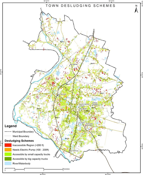
Figure 7 Illustrations of town desludging schemes based on hard-to-reach area findings, Sherpur (Bangladesh)

Source – CWIS spatial analysis, Innpact Solutions and GWSC

Output Application

The output here provides a clear understanding of the settlements accessible by large and small volume trucks. It pinpoints areas requiring additional infrastructure such as pipes and electric pumps and identifies inaccessible areas where manual or electric small carts are necessary for mechanical desludging.

As for its application, such framework can be instrumental in designing a desludging scheme for any towns. It aims to ensure a 100% safe collection mechanism for all users, effectively integrating data, analysis, and visualization to assist in efficient decisionmaking and strategy formulation for sludge emptying and collections.

Assessments of Waterlogging/Flood Prone Settlements

Data Requirements

1. Elevation data
2. Waterbodies/ Rivers
3. Past Flood data with location
4. High Flood Line for rivers

Stepwise Process Flow Details

• Step 1: Import Data o Open QGIS and load your Digital Elevation Model (DEM) data representing the topography of the study area. o Import building data and any other relevant spatial data layers, such as rivers, flood-prone areas, and historical flood level data, if available.

• Step 2: Clip the Digital Elevation Model o Use the "Clip raster by extent" tool to clip the DEM to your study region. This tool can be found in the Processing Toolbox (Processing > Toolbox) under the GDAL > Raster extraction menu.

• Step 3: Reclassify the DEM o Utilize the "Reclassify by table" tool in the Processing Toolbox (Processing > Toolbox) under the SAGA > Raster tools menu.

  o In the tool dialog, select the clipped DEM as the input raster, and define your flood threshold values in a reclassification table (e.g., set values less than the High Flood Line (HFL) to 1 and the rest to 0).

• Step 4: Identify Flood-Prone Areas o After reclassifying the DEM, the resulting raster image will represent potential flood-prone areas, where cells with a value of 1 are susceptible to flooding.

• Step 5: Use Historical Flood Levels (if available) o If you have access to historical flood level data, repeat Steps 2 and 3 with this data to create an additional raster representing historical flood-prone areas.

• Step 6: Overlay Buildings o Add the building data to QGIS and ensure it aligns correctly with the other layers. o Use the "Intersect" tool in the Processing Toolbox (Vector overlay > Intersection) to overlay the buildings layer with the flood-prone areas layer. This will help identify buildings falling within the flood-prone regions.

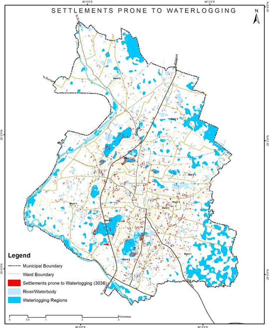
Figure 8 Illustrations of identifying of water logging prone settlements, Sherpur (Bangladesh)

Source – CWIS spatial analysis, Innpact Solutions and GWSC

Output Application

Assessment of Drainage Network with Orders and Density

Data Requirements

1.     Elevation data

2.     Waterbodies/ Rivers

Stepwise Process Flow Details

Step-by-step instructions in paragraph form for identifying natural drainage network and catchment areas from DEM using QGIS Hydrology tools:

• Step 1: Load the DEM for the Study Area o Open QGIS and add the DEM layer to your project by navigating to

  'Layer' > 'Add Layer' > 'Add Raster Layer'. Browse and select your DEM file.

• Step 2: Clip the DEM o To clip the DEM to a region larger than the study area, go to 'Raster' > 'Extraction' > 'Clip Raster by Extent'. o Select your input DEM layer and define the extent to cover an area larger than your study region.

  • Set the output file and click 'Run'.

• Step 3: Fill and Interpolate Gaps in the DEM and generate Flow Direction Raster o Install the 'SAGA' processing provider if you haven't already. Go to 'Processing' > 'Toolbox'. o In the processing toolbox, search for 'Fill Sinks (Wang & Liu)' and run the tool. o Select the clipped DEM as the input, set the 'Output corrected DEM' file, and run the tool.

  • This will generate both Filled DEM and Flow direction raster files

• Step 5: Generate the Stream Network o In the processing toolbox, search for 'Flow Accumulation' and run the tool. o Choose the flow direction grid (generated in the previous step) as the input and set the 'Flow accumulation grid' as the output.

• Step 6: Use the Raster Calculator Tool o In the processing toolbox, search for 'Raster Calculator' and run the tool. o Enter the expression to select pixels greater than a certain threshold (e.g., 5% of the maximum flow accumulation value). o Example: "flow_accumulation@1 > 0.05 * max_flow_accumulation_value" (Replace

  'max_flow_accumulation_value' with the actual maximum value). o Set the output raster file and run the tool.

• Step 7: Define the Stream Order o In the processing toolbox, search for 'Strahler Stream Order' and run the tool. o Choose the flow direction grid and the stream network raster (generated in the previous step) as inputs. o Set the output file and run the tool.

• Step 8: Convert to Polygon o In the processing toolbox, search for 'Raster to Polygon' and run the tool. o Select the stream order raster (generated in the previous step) as the input and set the output file.

• Step 9: Generate the Drainage Network o The stream polygons obtained from the previous step represent the drainage network classified according to stream order.

• Step 10: Create a New Shapefile o To delineate catchment areas and outfall locations, you can use a combination of 'Raster Calculator' and 'Raster to Polygon' tools to extract catchment boundaries from the flow accumulation raster. Then, manually digitize outfall points as new vector points in a new shapefile.

With these steps, you will be able to identify the natural drainage network and catchment areas from the DEM data using QGIS.

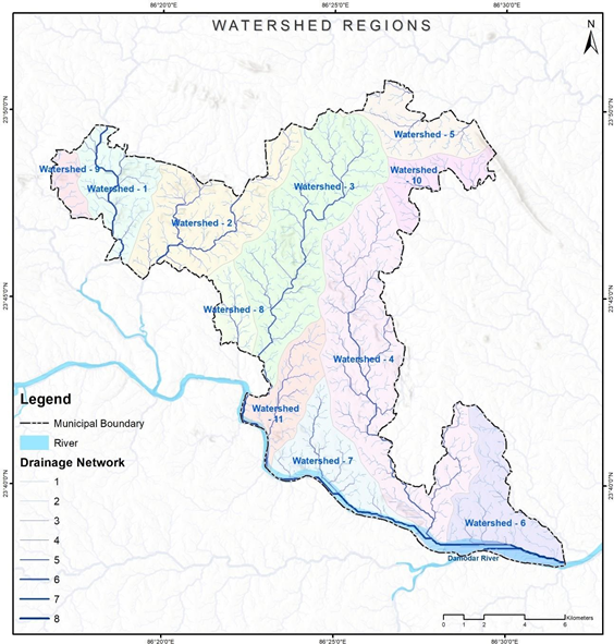
Figure 9 Illustrations of watershed regions at Dhanbad (India)

Source – CWIS spatial analysis, Innpact Solutions and GWSC

Output Application

A drainage network map helps delineate the different watersheds within a region, which play a significant role in both sewer and non-sewer zoning for any large town. Furthermore, watershed zones have significant applications in grey water management using an interceptor and diversion (I&D) framework. They can serve as functional linkages with the sewer system or may also operate as independent modules. Further this also has applications in identifying water logged prone area within the city. 

Assessment for Identifying Settlements Close to Waterbodies

Data Requirements

• Waterbodies/ Rivers

• Building footprint

Stepwise Process Flow Details

Stepwise Process Flow Details

• Step 1: Overlay the Data Layers

  Start by overlaying the water bodies, rivers, and building data layers on your map in the QGIS software. This involves using the 'Add Layer’ feature to import the necessary layers into your map document. Ensuring that all these layers are on the same coordinate system is crucial for achieving accurate results.

• Step 2: Conduct Buffer Analysis

  Next, perform a buffer analysis around the water bodies and rivers. Use the 'Buffer' tool within the ‘Vector Geometry’ section of the ‘Processing Toolbox’ menu. For water bodies, create a buffer of 30 feet and for rivers, create a buffer of 100 feet. This process essentially draws a boundary around the specified features (in this case, water bodies and rivers) at a set distance.

• Step 3: Identify Buildings within Buffer Regions

  Having established your buffer zones, it's now time to identify the buildings within these areas. To do this, use the 'Select by Location' tool. This tool allows you to select features (in this case, buildings) based on their geographic relationship to features within another layer (in this case, the buffer zones). Ensure you select the buildings that fall within the buffer regions that you created in the previous step.

• Step 4: Categorize Buildings

  Finally, classify all buildings that have been identified within the buffer regions as 'Water Proximity Buildings'. This can be done by creating a new field in the attribute table of the building layer and assigning these buildings with a specific tag or code.

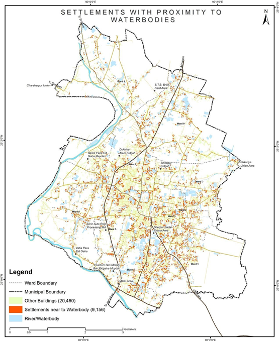
Figure 10 Illustrations for identifying settlements close to water bodies, Sherpur

Source – CWIS spatial analysis , Innpact Solutions and GWSC

Output Application

Areas in proximity to water tend to have a heightened risk of untreated wastewater encroaching into nearby water bodies, which can have significant public health and environmental ramifications. Identifying such settlements can guide the selection of safe containment provisions in both existing and upcoming units. These units can also be integrated with building by-laws and ensure safe containment provisions in all future constructions. 

Assessments for Identifying Economic Vulnerability Assessment

Data Requirements

1. Building footprint with Typology
2. Slum boundary

Stepwise Process Flow Details

• Step 1: Determine the Building Typology

  The first step involves examining the building data you've collected. If the data includes information on building typology, you can use this to identify all buildings with 'kutcha' construction - a term used in South Asia to refer to buildings made from materials such as mud, thatch, or bamboo. These structures are typically associated with economically vulnerable households.

• Step 2: Use Slum Boundaries

  If the building typology data is not available, you can use slum boundaries as an indicator of economically vulnerable settlements. Slums are often characterized by overcrowded and inadequate housing conditions and can be an indicator of economic vulnerability. If you have this boundary data, overlay it onto your existing map in the GIS software.

• Step 3: Conduct Overlay Analysis

  Having established the criteria for economic vulnerability (either kutcha construction or location within slum boundaries), perform an basic overlay analysis by using the tool, ‘select by location’ in QGIS software.

• Step 4: Categorize Buildings

  The final step is to categorize the buildings or settlements identified through the overlay analysis as 'Economically Vulnerable Settlements'. This can be done by creating a new field in the attribute table of the building layer and assigning these buildings with a specific tag or code.

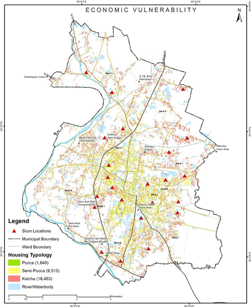
Figure 11 Illustrations for identifying economic vulnerable settlements, Sherpur (Bangladesh)

Source – CWIS spatial analysis, Innpact Solutions and GWSC

Output Application

Settlements identified as economically vulnerable are given priority when designing and implementing sanitation interventions across the sanitation value chain. These settlements can also be overlaid with other environmental and climate risk outputs to identify those with a higher degree of vulnerability.

Assessment for Settlement Identification for Bulk Volume of Wastewater Generation

Data Requirements

1. Building with type of use and number of floors

Stepwise Process Flow Details

• Step 1: Gather Building Data

  The initial step in the process involves gathering the relevant building data. This includes a building-level land-use map which details the characteristics of each building such as its type (e.g., residential, institutional), the number of floors it has, and other relevant data.

• Step 2: Import Data into GIS

  Import this data into your QGIS document. Make sure the data is correctly georeferenced to ensure accurate analysis.

• Step 3: Identify Key Buildings

  Next, use a selection query to identify key buildings that are likely to generate large volumes of wastewater. This includes high-rise buildings (those with more than three floors), apartment complexes, and institutional buildings such as residential schools, colleges, and hospitals.

• Step 4: Categorize Buildings

  Having identified these key buildings, categorize them as 'Bulk Wastewater Generators'. You can create a new field in the building layer's attribute table for this category, and assign each of the identified buildings to this new category.

• Step 5: Visualize and Analyze

  Finally, visualize these buildings on the map for a clear understanding of their distribution across the city. This could involve using different colors or symbols to represent the different categories of buildings. Analyze the spatial pattern of these buildings for insights into the bulk wastewater generation in the city.

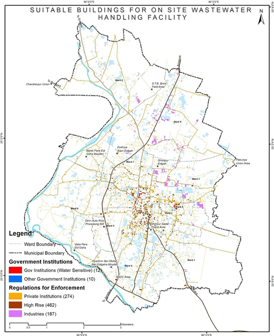
Figure 12 Illustrations of identifying settlements of bulk wastewater volume generator, Sherpur (Bangladesh)

Source – CWIS spatial analysis, Innpact Solutions and GWSC

Output Application

Buildings that produce significant wastewater should be prioritized for on-site treatment, particularly if they're near water-sensitive areas, given the considerable environmental and health risks. Recognizing these bulk generators can guide us in two ways. For government buildings, we can suggest interventions and financial aid to establish on-site wastewater systems. For private buildings, regulation and monitoring can gradually improve conditions. Including these generators in building bye-laws ensures future buildings consider wastewater management, promoting both immediate and long-term improvement

Assessment for Containment Improvement Scheme at Town Scale

Data Requirements

1. Output map of settlement near to water bodies,
2. Output map of settlement with waterlogged and flood prone risk
3. Output map of hard-to-reach settlement area
4. Output map of bulk wastewater generator building

Stepwise Process Flow Details

• Step 1: Gather Spatial Layers of Containment Risk This initial step involves the collection of spatial layers that map various types of containment risks. These might include data on settlements near water bodies, waterlogged areas, flood-prone regions, hard-to-reach settlements, and locations of bulk wastewater generators.
• Step 2: Overlay Risk Layers on City Building Footprints Once the necessary spatial layers have been collected, these layers can be overlaid on a city-wide map of building footprints. This process visualizes the proximity of each building to the various containment risks identified in Step 1. GIS software like QGIS is typically used for this process.
• Step 3: Understand City-Wide Risk at Building Level After the risk layers have been overlaid on the building footprints, it is possible to start understanding the distribution of risks across the city. Different color codes can distinguish between safe zones and risk areas. Within the risk areas, further categorization by typology can highlight different levels or types of risks. This may include different colors or symbols for buildings that are close to water bodies, located in flood-prone areas, hard to reach, or generate large amounts of wastewater. This city-wide risk understanding will provide a comprehensive view of the containment challenges at the building level.

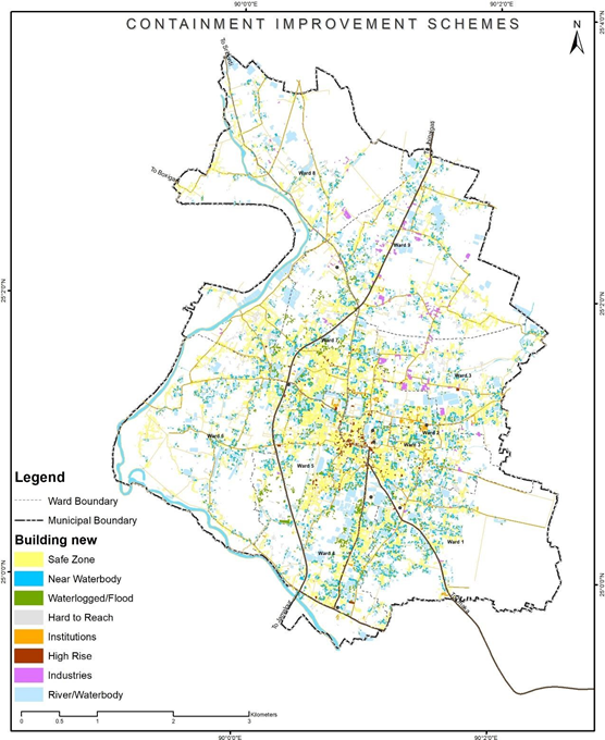
Figure 13 Illustrations of developing containment improvement scheme, Sherpur (Bangladesh)

Source – CWIS spatial analysis, Innpact Solutions and GWSC

Output Application

Location-based information can assist in tracking the evolution of improved containment systems over time. Such data also offers crucial insights for shaping city sanitation regulations, thereby facilitating an understanding of overall containment improvement objectives and designing service-level benchmarks for ongoing monitoring. Moreover, this information can be integrated with building bye-laws to ensure the selection of contextually appropriate containment systems in all future construction projects.

Assessments for Public Toilet Gap and Required Upgrades

Data Requirements

1. Major commercial and institutional land uses
2. Network Dataset using the road network layer
3. Location of public toilets with number of seats

Stepwise Process Flow Details

• Step 1: Assess the Walkability Factor

  For this process, a network analysis of the study region is necessary. This involves the creation of a network dataset.

• Step 2: Create a Network Dataset

  The road network shapefile must be clean and free from any topology errors.

  After ensuring the integrity of the shapefile, create a network dataset. o Ensure you have the "QNEAT3" plugin installed in your QGIS.

  o Load your road network shapefile in QGIS. o Use the "QNEAT3 > Create Network from Layer" tool to create a network dataset.

  This will initiate the creation of a network dataset using the road layer.

• Step 3: Conduct a Proximity Study

  Use the "QNEAT3 > Service Area (from Layer)" tool to conduct a proximity study using the locations of existing public toilets as input data.

• Step 4: Create a Network Buffer

  For each public toilet, create a network buffer representing a walkability distance of 500 feet.

  Step 5: Overlay the Data with Commercial Land Use

  Use the "Vector > Geoprocessing Tools > Intersect" tool to overlay the buffer data with the commercial land use data. This will help you identify major commercial areas and public places outside the walkability region of the public toilets.

• Step 6: Identify New Toilet Locations

  Based on the overlay analysis, pinpoint potential locations for new toilets. These should be in areas currently underserved by the existing public toilets, particularly in commercial and high traffic areas.

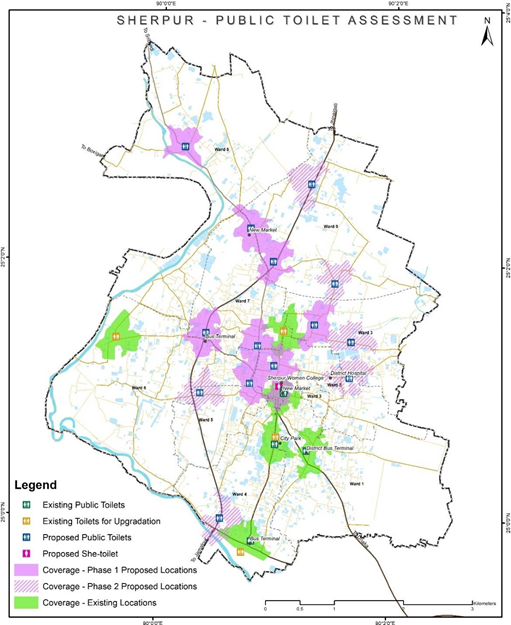
Figure 14 Illustrations of public toilet assessment of Sherpur, Bangladesh

Source – CWIS spatial analysis, Innpact Solutions and GWSC

Output Application

Implementing and adapting these recommendations would contribute to an adequate distribution and coverage of public toilet services throughout the city. A primary focus is on achieving a balanced gender distribution of water closets (WCs). Common observations across various cities have revealed a significant shortage of women's facilities in public toilet premises. Therefore, alongside general upgrades, there is a proposal to establish dedicated 'She Toilets' in high footfall areas to meet this demand.

Assessment of Pan City Level Settlements Proximity to Existing and Proposed FSTP

Data Requirements

1. Location of existing and proposed FSTPs
2. Network dataset using the road network layer

Stepwise Process Flow Details

• Step 1: Load the Network Dataset

  Load the road network shapefile in QGIS, which you created earlier as a network dataset.

• Step 2: Add FSTP Locations

  Add the locations of the existing and proposed FSTPs as input data for the network analysis.

• Step 3: Create Network Buffers

  To create network buffers representing travel times of 15 minutes, 30 minutes, and greater than 30 minutes for truck travel from each FSTP, you can use the "QNEAT3 > Service Area (from Layer)" tool. Select the FSTP locations as the input points. Configure the travel time intervals (15 minutes, 30 minutes, and greater than 30 minutes). Run the tool to create the network buffers centered on the FSTP locations.

• Step 4: Overlay Buffers on Settlement Data

  Overlay the network buffers onto the settlement dataset. This can usually be accomplished by using an 'Overlay' or 'Intersect' function within your GIS software.

• Step 5: Overlay Buffers on Settlement Data

  Overlay the network buffers onto the settlement dataset by using the "Vector > Geoprocessing Tools > Intersect" tool in QGIS.

  Select the settlement dataset as the input layer and the network buffers as the overlay layer. Run the tool to create a new layer containing the intersected features.

• Step 6: Identify Buildings within Buffers

  Identify and categorize the buildings within each buffer zone using the "Vector > Research Tools > Select by Location" tool in QGIS.

  Select the buildings layer as the target layer.

  Choose the buffer zones (15-minute travel time, 30-minute travel time, and greater than 30-minute travel time) as the source layer.

  Select the "Intersect" spatial selection method to find buildings within each buffer zone. Create a new layer with the selected buildings for each buffer category.

• Step 7: Calculate Percentages

  Calculate the percentage of buildings accessible within each of the buffer categories.

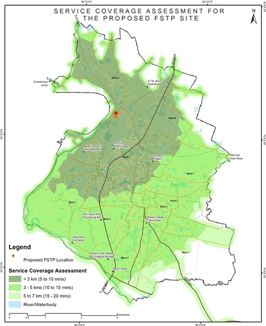
Figure 15 Illustrations of assessment of settlements proximity of proposed and existing FSTP, Sherpur (Bangladesh)

Source – CWIS spatial analysis, Innpact Solutions and GWSC

Output Application

This type of analysis aids in assessing the locational suitability of both existing and proposed Faecal Sludge Treatment Plant (FSTP) sites. Based on the results, areas outside of smooth travel distances might consider the possibility of implementing transfer stations or additional treatment facilities, contingent on the volume of sludge generated from their respective settlement areas. This spatial understanding provides a comprehensive approach for faecal sludge management planning and implementation across the city.