Stepwise Process Flow Details

• Step 1: Import Data o Open QGIS and load your Digital Elevation Model (DEM) data representing the topography of the study area. o Import building data and any other relevant spatial data layers, such as rivers, flood-prone areas, and historical flood level data, if available.

• Step 2: Clip the Digital Elevation Model o Use the "Clip raster by extent" tool to clip the DEM to your study region. This tool can be found in the Processing Toolbox (Processing > Toolbox) under the GDAL > Raster extraction menu.

• Step 3: Reclassify the DEM o Utilize the "Reclassify by table" tool in the Processing Toolbox (Processing > Toolbox) under the SAGA > Raster tools menu.

  o In the tool dialog, select the clipped DEM as the input raster, and define your flood threshold values in a reclassification table (e.g., set values less than the High Flood Line (HFL) to 1 and the rest to 0).

• Step 4: Identify Flood-Prone Areas o After reclassifying the DEM, the resulting raster image will represent potential flood-prone areas, where cells with a value of 1 are susceptible to flooding.

• Step 5: Use Historical Flood Levels (if available) o If you have access to historical flood level data, repeat Steps 2 and 3 with this data to create an additional raster representing historical flood-prone areas.

• Step 6: Overlay Buildings o Add the building data to QGIS and ensure it aligns correctly with the other layers. o Use the "Intersect" tool in the Processing Toolbox (Vector overlay > Intersection) to overlay the buildings layer with the flood-prone areas layer. This will help identify buildings falling within the flood-prone regions.

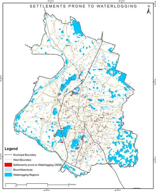
Figure 8 Illustrations of identifying of water logging prone settlements, Sherpur (Bangladesh)

Source – CWIS spatial analysis, Innpact Solutions and GWSC